Introduction
The indication of layer-thickness by apparent conductivity is a
long-standing application of low-induction-number electromagnetic (LIN EM)
surveys. For example, Müllern, et al. (1983) used apparent
conductivity from a 3.7-m horizontal co-planar (HCP) array as a linear
indicator of the thickness of glacial sediments over crystalline bedrock.
The popularity of the interpretation of apparent conductivity as a linear
indicator of thickness results from the reasonable results it proves in some
cases, and its computational convenience.
Forward modeling of LIN EM response can outline conditions suited to
such interpretation.
Simple transformation of the apparent-conductivity values can improve the
linearity between apparent conductivity and thickness of surficial material,
but such transformations tend to amplify irregularities that cause
interpretational uncertainty.
Conductive Layering and Apparent Conductivity
Conductive layering in the near surface results from a number of conditions that are of interest to a variety of surveyors. The thickness of soil to bedrock often has agricultural and geotechnical significance.
Soil that develops from underlying bedrock is generally more conductive than the bedrock. Transported soil can contrast with bedrock that is either very resistive or conductive. A layer of frozen soil tends to be much less conductive than unfrozen soil beneath it. Ice contrasts very strongly in conductivity with seawater, and can be substantially less conductive than lakes and rivers that have significant levels of dissolved solids.
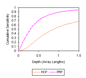
LIN EM is suitable for identifying conductive layering within the depth of exploration (DOE) of the EM array. A widely accepted guideline for DOE is the depth at which the LIN EM array has accumulated 70 % of its sensitivity. The cumulative-sensitivity functions for popular arrays (Taylor, 1999) are illustrated in Figure 1.
Where the unit of depth is the distance, d, between the transmitter and receiver of the array, the DOE of the perpendicular (PRP) array is about 0.5 d, and the DOE of the horizontal co-planar (HCP) array is about 1.5 d.
The functions of cumulative sensitivity are approximately linear with depth to the DOE. This suggests that apparent conductivity, which is proportional to the sensitivity accumulated through a layer times the conductivity of the layer, should be an approximate indicator of the thickness of the layer if the conductivity is constant.
Figure 1:
Cumulative Sensitivity versus Depth.
Models of Response
Even where layer-conductivity is constant, complicating factors for apparent conductivity are the sensitivity to the depth of air between the EM array and the earth (as the array is carried above the surface), and the contrast between the conductivities of the layer and the underlying earth.
The following forward models of LIN EM response show the relationship between layer thickness and apparent conductivity for different heights and contrasts. In each case, the linearity of the relationship to the DOE is indicated by a correlation coefficient. The coefficient is calculated using a number of discrete values of apparent conductivity evenly spaced over the DOE.
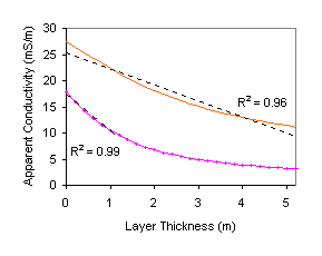
Figures 2 and 3 show apparent conductivities that will be measured by a DUALEM-2 (2-m dual HCP/PRP array) at 0.1-m height. This height is representative of surveys where the array is mounted in a sled or low cart. The thickness of the surficial layer varies from 0- to 3-m.
For Figure 2, the conductivity of the surficial layer is 30 mS/m, and the conductivity of the underlying earth is 3 mS/m. Conductivities such as these might be encountered where medium-textured soil overlies limestone (or other fairly resistive bedrock).
Figure 2:
DUALEM-2 and Conductive Layer.
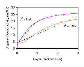 The correlation coefficients of 0.96 and 0.98 confirm that
the relationship between apparent conductivity and layer thickness is highly
linear to the DOE. Beyond the DOE,
apparent conductivity will increasingly under-indicate thickness, as shown by
the flattening of the PRP curve for thickness greater than 1 m.
The correlation coefficients of 0.96 and 0.98 confirm that
the relationship between apparent conductivity and layer thickness is highly
linear to the DOE. Beyond the DOE,
apparent conductivity will increasingly under-indicate thickness, as shown by
the flattening of the PRP curve for thickness greater than 1 m.
The PRP curve is relatively steep within its DOE, so PRP apparent conductivities are more sensitive to changes in thickness to about 1 m. The greater DOE of the HCP provides a linear indication of thickness to about 3 m. Under these conditions, the apparent conductivities range through about 19 mS/m within the DOE. Conductivity fluctuations equivalent to a significant fraction of this range in material that occupies a substantial portion of the DOE will confound the linear interpretation of layer thickness from apparent conductivity.
For Figure 3, the conductivity of the surficial layer is 3 mS/m, and the conductivity of the underlying earth is 30 mS/m. Conductivities such as these might be encountered where coarse-textured soil overlies clay, or soil saturated with brackish pore-fluid.
Figure 3: DUALEM-2 and Resistive Layer.
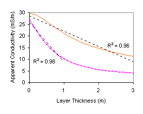 With allowance for the inverse relationship between the
thickness of a resistive layer and apparent conductivity, the linearity and
range of values are essentially similar to those illustrated by Figure 2.
With allowance for the inverse relationship between the
thickness of a resistive layer and apparent conductivity, the linearity and
range of values are essentially similar to those illustrated by Figure 2.
Figures 4 and 5 show apparent conductivities that will be measured by a DUALEM-4 (4-m dual HCP/PRP array) at 0.9-m height. This height is representative of surveys where the array is carried near the hip of the surveyor. The thickness of the surficial layer varies from 0 m to about 5 m. (Note that, in addition to the layer and underlying earth, there is also 0.9 m of air within the DOE.)
For Figure 4, the conductivity of the surficial layer is 30 mS/m, and the conductivity of the underlying earth is 3 mS/m.
Figure 4: DUALEM-4 and Conductive Layer.
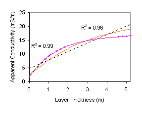 The correlation coefficients show that the linearity between
thickness and apparent conductivity remains high for this situation. Compared to the ranges of apparent
conductivity for the DUALEM-2 close to the earth, the range for HCP apparent
conductivity in Figure 4 is slightly diminished, and the range for PRP is
substantially diminished. The diminished range makes conductivity fluctuations
slightly more problematical to the interpretation of thickness.
The correlation coefficients show that the linearity between
thickness and apparent conductivity remains high for this situation. Compared to the ranges of apparent
conductivity for the DUALEM-2 close to the earth, the range for HCP apparent
conductivity in Figure 4 is slightly diminished, and the range for PRP is
substantially diminished. The diminished range makes conductivity fluctuations
slightly more problematical to the interpretation of thickness.
For Figure 5, the conductivity of the surficial layer is 3 mS/m, and the conductivity of the underlying earth is 30 mS/m.
Figure 5: DUALEM-4 and Resistive Layer.
 With allowance for
the inverse relationship between the thickness of a resistive layer and
apparent conductivity, the linearity and range of values are essentially
similar to those illustrated by Figure 4.
With allowance for
the inverse relationship between the thickness of a resistive layer and
apparent conductivity, the linearity and range of values are essentially
similar to those illustrated by Figure 4.
Thus, for LIN EM arrays at heights above the earth commonly used for surveying, measurements of apparent conductivity have similar ability to indicate of the thickness of either a conductive or resistive layer.
Measurement Transformation
The shape of the curves of apparent conductivity suggests that simple transformation of these values would improve the linearity of the relationship with layer thickness. For example, using the same array-height and conductivities as for Figure 5, Figure 6 graphs the inverse of the square-root of apparent conductivity versus thickness.
Figure 6: Resistive Layer with Transformation.
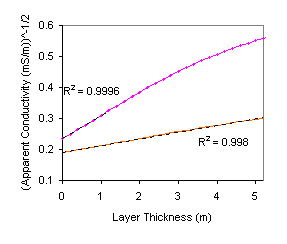 This transformation, however, effective squares the error due
to conductivity fluctuation, which more than negates the improvement in
linearity.
This transformation, however, effective squares the error due
to conductivity fluctuation, which more than negates the improvement in
linearity.
Conductivity Fluctuation
Figure 7 illustrates the uncertainty that arises from fluctuations in conductivity. The figure shows the same curves as Figure 2, but with error bars that show the variation in apparent conductivity that would be caused by 20-% fluctuations in conductivities of the surficial layer and the underlying earth. That is, the upper limit of the error bars shows the apparent conductivities for a 36-mS/m layer and a 3.6-mS/m earth, the lower limit shows the apparent conductivities for a 24-mS/m layer and a 2.4-mS/m earth.
Figure 7: Fluctuation in Conductivity.
 Where thickness approaches the DOE, flattening of the curves
along with increasing deviation from the curves due to conductivity fluctuation
makes indication of thickness unreliable.
With 20-% fluctuation around an order-of-magnitude conductivity
contrast, as shown here, thickness indication appears to limited to less than
one-half the nominal DOE. Indication to
greater thickness is feasible where the contrast is greater (i.e. the curves
are steeper), and where conductivities are highly consistent.
Where thickness approaches the DOE, flattening of the curves
along with increasing deviation from the curves due to conductivity fluctuation
makes indication of thickness unreliable.
With 20-% fluctuation around an order-of-magnitude conductivity
contrast, as shown here, thickness indication appears to limited to less than
one-half the nominal DOE. Indication to
greater thickness is feasible where the contrast is greater (i.e. the curves
are steeper), and where conductivities are highly consistent.
Conclusions
Apparent conductivity measured by LIN EM arrays can be linear indicator of the thickness of a surficial layer to the DOE. The large DOE of the HCP array makes its measurements preferable for greater thickness, and the sensitivity of the PRP array makes its measurements preferable for lesser thickness.
The sensitivity of the HCP array will diminish slightly as the surveying height increases to the maximum commonly used, and the sensitivity of the PRP array will diminish substantially.
The surficial layer can be either conductive or resistive, relative to the underlying earth. The contrast in conductivity between the layer and earth should be much larger than conductive fluctuations within either unit. For example, where the contrast is an order-of-magnitude, fluctuations should not exceed, say, 20 %.
The accuracy of the thickness indication will increase with the conductivity contrast between the layer and the underlying earth, provided that the minimum level of apparent conductivity exceeds the noise level of the survey.
References
C.R. Müllern, L. Eriksson and Ch. Persson (1983), “Electromagnetic Measurements for Continuous or Local Assessment of Depths and Types of Quaternary Deposits in Profiles,” in Proceedings, International Symposium on Engineering Geology and Underground Construction, Lisboa, 1983 (Lisbon: Sociedade Portuguesa de Geotechnica, 1983), I, 71-80.
R.S. Taylor (1999), "A History of the Development and Applications of Geometric-Sounding EM Instruments," www.dualem.com/gsem.htm.