Table of Contents
Introduction
The electrical conductivity of geological materials varies over many orders of magnitude, and most materials have distinctive ranges of conductivity. Electromagnetic induction (EMI) is an effective technique for measuring electrical properties but, in general, is complex in operation and interpretation.
Compact devices greatly simplify EMI, in that they are most portable and operate typically at low induction number (LIN). With relative ease, LIN data yield reliable interpretations of the conductivity and spatial extent of geological materials.
Electrical Conductivity
The siemen, S, is the SI unit of conductance. Also known as the mho (i.e. inverse of ohm), the siemen is defined as A/V, where A is the current in amperes that flows in an electric circuit when a voltage V, in volts, is applied.
An electrical circuit in the earth has a cross-sectional area through which the current flows, and a length over which the voltage is applied. For a measure that is independent of circuit dimensions, we divide current by area and voltage by length (i.e. A/m2 / V/m) and obtain S/m, which is the SI unit of conductivity.
The following chart (after Palacky, 1987) shows that the conductivities of geological materials span many orders of magnitude, and that a convenient unit for terrain conductivity is the millisiemen per metre, or mS/m.
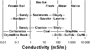
The upper portion of the chart shows conductivities of the various forms of water and of frozen soil, the conductivity of which is governed by the ice it contains. Unconsolidated materials, both transported and residual, are found in the central level of the chart, below which are lithified materials.
Geological materials that are moist typically conduct current through the movement of ions. The ions may be in solution, or associated with surficial charges of some clays, etc. The conductivity of moist material shows linear proportionality to its temperature. The seasonal effect of temperature fluctuations in a moderately conductive material is typically several mS/m. Freezing a material tends to drop its conductivity exponentially, usually by at least one order of magnitude.
Native metals, sulfides and graphite conduct current through the movement of electrons. With such materials, conductivity shows a small inverse proportionality to temperature.
Electromagnetic Induction
EMI instruments transmit a primary magnetic field, which induces electrical current in the earth. The current in the earth generates a secondary magnetic field, which is sensed by the receiver of the instrument. The characteristics of the secondary field indicate the conductivity of the earth.
EMI techniques are distinguished by the nature of the primary field. Transient (or time-domain) EMI uses an intermittently pulsed primary field, and measures the change in the secondary field at various times between pulses. Continuous (frequency-domain and LIN) EMI uses a continuously varying primary field, and measures the amplitude and phase of the secondary field relative to the primary field.
Most continuous EMI instruments transmit sinusoidal primary fields at a fixed frequency, as depicted in the following figure. Such transmission is efficient, which facilitates the acquisition of accurate data with instrumentation that is relatively light and compact. The figure also shows a secondary field that represents the response of an earth that contains conductive material.
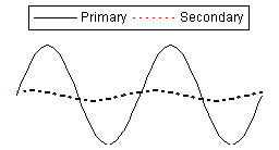
The amplitude of the secondary field at the receiver is normalized to the amplitude of the primary field at the receiver, in units such as percent, parts-per-thousand (ppt), etc. The phase of the secondary field is also compared to that of the primary field.
Figure 3 is a portion of Figure 2, stretched to show phase components of the secondary field. The in-phase component coincides with the peak of the primary field, and the quadrature component leads the in-phase component by one-quarter cycle, i.e. 90 degrees.
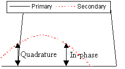
In this example, the secondary field leads the primary field by about 45 degrees, so the in-phase and quadrature amplitudes are about equal.
Transmitter-receiver geometry is an essential aspect of EMI. Geometry is the orientation and separation of the transmitter (Tx) and receiver (Rx) relative both to each other and to the earth. DUALEM instruments combine two geometries, usually called “horizontal co-planar” (HCP) and “perpendicular” (PRP). The following figure shows a schematic profile of a DUALEM instrument.
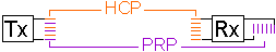
A DUALEM instrument uses bobbin-wound coils for its Tx and Rx. For the HCP geometry, the windings of the Tx- and Rx-coils lie in the same horizontal plane. The PRP geometry shares the same Tx, but the windings of its Rx coil are vertical, and axis of the coil intersects the Tx.
The Tx-Rx separation is 2 m for the DUALEM-2, and 4 m for the DUALEM-4. (As the separations are more than several times as large as the coil diameters, each coil can be treated mathematically as an oscillating magnetic dipole that is aligned with the coil axis.)
To illustrate the significance of geometry, the following figure shows schematic profiles at four critical points of a DUALEM traverse over a thin-and-shallow conductor. The senses of current in the conductor and in the DUALEM coils are shown by the triangles on these features. Triangles also show the senses of the magnetic flux of the primary and secondary fields. At each point, current in the edge of the Tx coil closest to us flows from right to left, which generates a primary field with a downward sense.
At the bottom of the figure are diagrammatic profiles that show the characteristics of continuous measurements across this type of conductor.
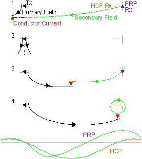
Profile 1 shows the DUALEM approaching the conductor. The leftward sense of the primary field that intersects the conductor induces current that, in the edge of the conductor closest to us, flows upward. This generates a secondary magnetic field with a similar sense through the conductor to that of the primary field.
The secondary field disperses away from the axis of the induced current, and some of its flux intersects the Rx coils. The downward sense of the flux induces current in the HCP Rx coil that, in the edge closest to us, flows from right to left. The leftward sense of the flux induces current in the PRP Rx coil that, in the edge closest to us, flows upward.
Relative to the Tx current, these Rx currents are considered to be positive, but they are weak due to the combined distance that the primary and secondary fields must travel, first to the conductor, and then to the Rx. Their values are shown qualitatively on the measurement profiles at the bottom of the figure, directly below the location of the conductor in profile 1.
Profile 2 shows the point at which the axis of the Tx is directly over the conductor. As the flux of the primary field disperses symmetrically about the Tx axis, no net amount of flux intersects the conductor, no current is induced, no secondary field is generated, and no current is induced in the Rx coils. The Rx values of zero are plotted on the measurement profiles, directly below the position of the conductor in profile 2.
Beyond the point of profile 2, the primary field has a rightward sense. This sense induces current in the conductor that, in the edge closest to us, flows downward.
Profile 3 shows the point at which the conductor is midway between the Tx and Rx. The downward sense of the conductor current induces a secondary field with a rightward sense. Some of the secondary flux disperses upward, develops an upward component to its sense, and intersects the Rx.
The upward sense of the flux induces current in the HCP Rx coil that, in the edge closest to us, flows from left to right. The rightward sense of the flux induces current in the PRP Rx coil that, in the edge closest to us, flows downward. The senses of these currents are opposite those in profile 1 and, thus, are deemed negative.
As shown on the measurement profiles, the most negative HCP value over a thin conductor generally occurs where the conductor is midway between the Tx and Rx. This is a consequence of the relatively short combined distance that the primary and secondary fields must travel, but also to the relatively strong upward component of the secondary flux at this point.
As the upward component increases, the rightward component decreases, which decreases the amplitude of the PRP value. The secondary flux is vertical where the PRP value passes through zero between the points of profiles 3 and 4.
Profile 4 shows the point at which the HCP Rx coil is directly over the conductor. The secondary field is horizontal above the conductor, so no net amount of flux passes through the HCP Rx coil and the HCP current is zero.
For practical purposes in DUALEM instruments, the PRP and HCP Rx coils are separated slightly. At the point of profile 4, the PRP Rx coil has not moved directly over the conductor, but the sense of the secondary flux through the coil is leftward, producing a positive value for the current. The PRP response reaches a maximum near the point directly over the conductor.
Beyond the point of profile 4, the HCP and PRP values generally decrease, as the combined distance increases through which the primary and secondary fields must travel.
Continuous responses of the types depicted here are commonly termed “shoulders-and-trough” for HCP, and “crossover” for PRP. Note that the depictions are qualitative, and that actual responses vary greatly in amplitude, phase, form and complexity with, among other factors, the conductance, depth and shape of the conductor and its situation relative to the survey path.
Lightning provides another graphic example of geometry. Lightning generates broadband electromagnetic energy in the atmosphere, which appears as noise in broadband EMI data. (DUALEM instruments are sensitive only to the small fraction of the energy that has an effective frequency equal to the 9-kHz DUALEM frequency.)
If we characterize lightning as a vertical pulse of electrical current, the current will transmit a horizontal magnetic field. Long-distance propagation of the field is enabled where a conductive earth (e.g. ocean) is present to complement the ionosphere in guiding the horizontal field. The following figure is a plan view of a lightning strike, its transmitted field, and the HCP and PRP geometries.
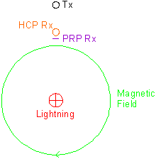
The effect of the horizontal magnetic field on the horizontal Tx and HCP Rx will be minimal, as little flux will intersect the coils. With the long axis of the PRP geometry oriented toward the lightning, as shown, little flux from the horizontal magnetic field will intersect the PRP Rx so the effect, again, will be minimal. Where the PRP geometry is oriented at right angles to the prevalent direction of atmospheric disturbance, however, noise in the PRP data may arise from distant disturbances if the intervening earth is conductive, and noise typically increases as the distance to the disturbance decreases.
Induction Number
The induction number (IN) characterizes the EMI of a homogeneous earth. The IN is defined as (cmw)1/2s, where c is the conductivity of the earth, m is the magnetic permeability of the earth, w is the angular frequency of the primary field and s is the transmitter-receiver separation.
For example the IN is about 0.084, where an instrument with 2-m separation operates at 9 kHz (2π x 9000 radians/s) on an earth with 25 mS/m (0.025 S/m) conductivity and free-space (4π x 10-7 H/m) magnetic permeability. Note that the IN is dimensionless.
The following figure shows the amplitudes of phase components of the secondary field that are measured by the HCP and PRP geometries at INs from 0 to 3.5. The markers on the curves show increments of 0.5 in the IN. The chart is drawn from data in Frischknecht (1967).
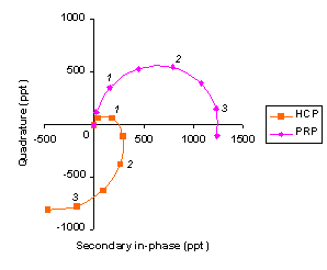
The phasor diagram provides a graphic summary of the effect of IN on the amplitude and phase of the secondary field. Near the origin, both the HCP and PRP curves show a steep positive slope, as quadrature amplitude increases rapidly with increasing, but low, induction.
As induction continues to increase, both components increase in amplitude, but the slopes of the curves start to flatten as the peak of secondary field begins to shift towards the in-phase component.
At INs of about 0.76 for HCP and 1.8 for PRP, the curves are horizontal. At these INs, the increase in quadrature due to increasing induction is balanced by the decrease in quadrature due to the shift of the secondary-field peak toward in-phase.
At INs of about 1.2 for HCP and 3.3 for PRP, quadrature has decreased to zero, as the secondary field has shifted to exact alignment with the in-phase component.
Also at an IN of about 3.3 for PRP, and about 1.7 for HCP, the curves become vertical. The secondary field has shifted beyond in-phase alignment, and the decrease in in-phase amplitude due to the shift balances the increase due to increasing induction.
The HCP curve passes through another notable point before reaching the maximum graphed IN of 3.5. At an IN of about 2.6, HCP in-phase is zero, as the secondary field has shifted to an alignment exactly opposite to quadrature.
The accurate measurement of phase components over a significant range of INs provides a basis for interpreting the extent of conductive layering in the earth. The following figure shows an example of such interpretation by Palacky (1991).
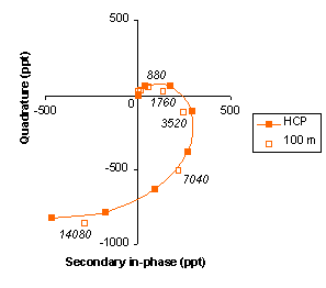
The figure shows again the curve for HCP measurements on a homogeneous earth for INs of 0 to 3.5, along with eight pairs of phase measurements (“100 m”). The measurements were made at the eight frequencies of 110-, 220-, 440-, 880-, 1760-, 3520-, 7040-, and 14080-Hz, using an HCP array with 100-m separation between the Tx and Rx. The separation was controlled within a tolerance of 0.2 m, which constrained the error of repeated measurements to about 10 ppt. Frequent calibrations were used to correct for drift.
The eight measurements conform fairly well to the curve for a homogenous earth. The measurement at 7040 Hz lies very close to the point of the curve with an IN of about 2.2. Using the formula IN = (cmw)1/2s, the measurement indicates a conductivity of about 9 mS/m for a homogenous earth.
Conductive layering in the earth is revealed by the pattern of the small deviations of the measurements from the curve. The measurement at 14080 Hz lies farther from the origin than the local part of the curve, while the 3 measurements below 7040 Hz, i.e. at 3520-, 1760- and 880-Hz, lie closer to the origin than the curve. (The measurements at 440 Hz and below are poorly resolved near the origin, and are not useful for interpretation.)
The deviations from the curve indicate that the earth seems more conductive than a homogeneous earth at the shallower-penetrating high frequency, while the earth seems less conductive at the deeper-penetrating lower frequencies. Thus, the deviations suggest that the upper earth is more conductive than the lower earth.
When the measurements are compared to model values for an earth with a surficial layer of 20-mS/m conductivity and 42-m thickness on underlying material of 0.1-mS/m conductivity, the measurements fit with an error of about 1 %. Such an earth corresponds well with a borehole at the measurement location, which reached crystalline bedrock beneath 35 m of glacial sediments.
Large Tx-Rx separations are a means of obtaining measurements at the range of INs necessary for multi-frequency sounding. However, spatial resolution coarsens as separation increases, which makes large separations impractical for sounding the uppermost 10 m of the earth.
Theoretically, it should be possible to sound shallowly with phase measurements from short Tx-Rx separations, provided that the measurement frequencies cover a substantial range of INs. Inspection of the IN formula, however, shows that this is generally impractical. For example, if we shorten the separation by a factor of 50, e.g. from 100 m to 2 m, we must broaden the frequency range by a factor of 2500, as IN is proportional to separation, but to only the square-root of frequency.
The following figure shows an attempt at multi-frequency sounding with an HCP instrument that has a Tx-Rx separation of 1.6 m. The figure shows the three pairs of phase measurements (“1.6 m”) made at 990-, 4470-, and 19950-Hz. The figure also shows the HCP curve for a homogeneous earth, with the IN range of 0 to 0.05.
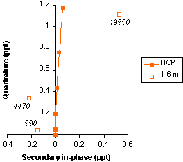
The scatter of the measurements arises from in-phase values that are unrealistic in sign and amplitude. The values indicate that errors in zero-level calibration are much larger than the in-phase responses of the earth, and that the errors vary incoherently from frequency to frequency.
In-phase error renders academic the question of the IN range covered by the frequencies. (For a range comparable to the previous example, the 1.6-m instrument would have to operate at frequencies up to 98 MHz, a frequency at which ground-penetrating-radar instruments operate using EM radiation, rather than EMI). More significantly, the scatter of the measurements causes the simple interpretation of homogeneous-earth conductivity from the multi-frequency data to become problematic.
EMI instruments with short Tx-Rx separations are generally incapable of measuring in-phase with interpretable accuracy, as the strength of the primary field at the Rx is inversely proportion to the cube of the separation. For example, the primary field at the Rx of a 1.6-m array is 244,000-times as strong as it is at the Rx of a 100-m array, and in-phase zero-level instability caused by expansion, contraction or bending of the array is amplified accordingly.
Less importantly, fluctuations in the magnetic susceptibility of shallow material will affect the stability of the in-phase component.
Low Induction Number
At LIN, Wait (1962) shows that nearly all of the conductive response from a homogeneous- or layered-earth is quadrature, so an inaccurate in-phase component can be ignored. Wait proposes that LIN conditions exist for the PRP geometry to an IN of about 0.5, where quadrature still accounts for about 99 % of total response. Using a similar criterion for the HCP geometry, LIN conditions exist to an IN of about 0.16.
Using these limits and assuming that the earth has the magnetic permeability of free space, LIN conditions exist for DUALEM-2 measurements where HCP conductivity does not exceed 90 mS/m, and PRP conductivity does not exceed 800 mS/m. The corresponding conductivities for the DUALEM-4 are 23 mS/m for HCP, and 210 mS/m for PRP.
Wait (ibid.) shows that conductivity at LIN is linearly proportional to quadrature, and describes the accumulation of PRP conductivity from a layered earth. McNeill (1980) describes the corresponding accumulation of HCP conductivity. These accumulations form the basis of interpreting conductive layering in the upper few metres of the earth from DUALEM measurements.
The PRP geometry accumulates its measurement of conductivity with depth proportionally to P(d)=2d/(4d2+1)1/2, where d is the depth beneath the instrument, in units of the Tx-Rx separation.
In the same units of Tx-Rx separation, the HCP geometry accumulates its measurement of conductivity proportionally to H(d)=1-1/(4d2+1)1/2.
The accumulation functions provide an indication of depth of exploration. For example, the PRP geometry accumulates 70 % of its total response within a depth equivalent to 0.5 coil-separations, and the HCP geometry accumulates similar response within 1.5 coil-separations.
Where there is conductive layering beneath the instrument, each geometry will measure a value of conductivity equal to the sum of the conductivity of each layer times the accumulation of response in that layer.
The following figure depicts a layered earth sounded by a DUALEM-4, where h is the height of the instrument above the earth, ca is the conductivity of the air, t is the thickness of an upper layer of the earth, ct is the conductivity of the upper layer, and c is the conductivity of the remainder of the earth.
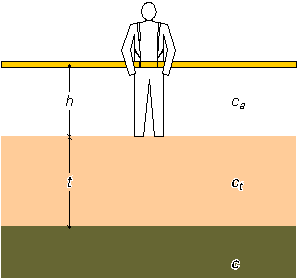
The PRP conductivity measured over this earth will be:
P = ca P(h) + ct (P(h+t) – P(h)) + c (P(∞) – P(h+t))
and the HCP conductivity will be:
H = ca H(h) + ct (H(h+t) – H(h)) + c (H(∞) – H(h+t)).
Since the conductivity of air is essentially zero, and the accumulation of response to infinity is 1, the expressions for apparent conductivity simplify to:
P = ct (P(h+t) – P(h)) + c (1 – P(h+t))
and
H = ct (H(h+t) – H(h)) + c (1 – H(h+t)).
If we know the height of measurement, and assign a thickness for the upper portion of the earth, we can calculate the various accumulations of response. This leaves us with two unknowns, ct and c, in two equations, which can be solved by the isolation and substitution of variables.
If we assign a value for the conductivity of either the upper- or the underlying-earth, we should be able to solve for the other conductivity and the thickness of the upper earth. However, the variable t is embedded in the accumulation functions in such a way that it is difficult to isolate or substitute. Nevertheless, where one of the conductivities can be fixed at a realistic value, approximate solutions for thickness and the other conductivity are sometimes satisfactory.
To increase confidence in an approximate solution, or to estimate values for more than two variables, measurements can be made at a number of heights. Such a procedure performed at a given location is called a vertical sounding.
The following figure shows DUALEM-2 measurements (HCP and PRP) from a vertical sounding, along with lines that show values calculated from the accumulation functions for both a homogeneous earth (HCP HE and PRP HE) and a layer on an underlying earth (HCP L+E and PRP L+E).
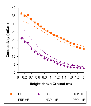
The HCP and PRP conductivities decrease with increasing height, as more of the responses accumulate in non-conductive air. The dashed lines show the values that should be obtained over this range of heights above a 32-mS/m homogenous earth.
The HCP geometry accumulates more of its response at greater depth than the PRP geometry. As the HCP measurements are greater than those for a 32-mS/m earth, and the PRP measurements are less, the sounding indicates the presence of a lower earth that is more conductive than 32 mS/m, under a less conductive surficial layer.
The solid lines show the values that should be obtained over a model earth with such layering. The model has a surficial layer of 1-mS/m conductivity and 0.55-m thickness, on an underlying earth of 44-mS/m conductivity.
While the presence of a surficial layer is indicated clearly by the vertical sounding, the parameters of the layer are poorly resolved. For example, a model with a layer of 5-mS/m conductivity and 0.65-m thickness on an underlying earth of 45-mS/m conductivity fits the measurements essentially as well as illustrated example.
The vertical sounding was taken over an earth with turf and topsoil on fine-grained subsoil that becomes rich in carbonate below a horizon of leaching.
The vertical sounding was made at the same location as the multi-frequency measurements of figure 9. The conductivities of the sounding confirm that the multi-frequency measurements were made at LIN, regardless of frequency.
At LIN, in-phase amplitudes are an insignificant fraction of total response. Since the in-phase values measured by the multi-frequency instrument are similar in amplitude to the quadrature values, they are spurious and useless in the interpretation of conductivity.
Indeed, it is noteworthy that short multi-frequency instruments that show measurements of apparent conductivity do so by scaling the values from the amplitude of the quadrature component, an interpretation that is valid only at LIN. It follows that if these measurements are valid, they must accumulate from depths defined by the LIN functions of Tx-Rx separation, regardless of the operating frequency of the instrument.
Summary
Many geological materials, including most soils and some bedrock, have conductivities that can be measured with EMI. Continuous EMI, which measures in-phase and quadrature responses with various Tx-Rx geometries, is an efficient technique both for profiling discrete conductors and for sounding conductivity.
Where Tx-Rx separation is large, measurements over a wide range of frequencies can be used to estimate the thickness and conductivity of contrasting layers in the earth. Where Tx-Rx separation is small, layer thickness and conductivity can be estimated from quadrature measurements using distinct geometries and measurement heights.
References
Frischknecht, F.C., 1967, Fields about an oscillating magnetic dipole over a two-layer earth, and application to ground and airborne electromagnetic surveys: Colorado School of Mines Quarterly, 62.
McNeill, J.D., 1980, Electromagnetic terrain conductivity measurement at low induction numbers: Geonics Ltd., Technical Note TN-6.
Palacky, G.J., 1987, Resistivity characteristics of geologic targets, in Nabighian, Misac N., ed., Electromagnetic Methods in Applied Geophysics (2 volumes): Society of Exploration Geophysicists, I, 53-129.
Palacky, G.J., 1991, Application of the multifrequency horizontal-loop EM method in overburden investigations, Geophysical Prospecting, 39, 1061-82.
Wait, J.R., 1962, A note on the electromagnetic response of a stratified earth: Geophysics, 27, 382-85.