ESTIMATING LAYERED-EARTH CONDUCTIVITY AND THICKNESS WITH MULTIPLE-ARRAY ELECTROMAGNETIC INSTRUMENTS
Richard S. Taylor
Dualem Inc.
Milton, Ontario
Canada
Abstract
Since 1999, dual-array electromagnetic (EM) instruments have been used to identify the presence of layering of electrical conductivity in the upper-few metres of the earth. Newly introduced instruments with multiple arrays can provide more detailed information about conductive layering. Examples and a simulation show that the detailed measurements from the multiple-array instruments can estimate the conductivity and thickness of a surficial layer, as well as the conductivity of the earth that underlies the layer.
Keywords: electromagnetic induction, EMI, electrical conductivity, layer thickness
Introduction
A type of EM instrument that has seen increasing use since 1999 in precision agriculture incorporates horizontal co-planar (HCP) and perpendicular (PRP) arrays that operate at very low frequency. The depth sensitivity of such arrays is a function of their length, i.e. the horizontal separation between their transmitter and receiver.
The annotations of Figure 1 show the essential configuration of an instrument with 1-m arrays. The transmitter-coil, shared by both arrays, has horizontal windings. The HCP receiver has windings that are horizontal and co-planar with those of the transmitter. The PRP receiver has windings that are vertical and perpendicular to the array axis.
Figure 2 shows the cumulative-sensitivity versus depth for the two arrays to electrical conductivity beneath them. The sounding depth of the PRP array is comparatively shallow, as the array develops half its sensitivity to a depth equivalent to about 0.3 array lengths. In contrast, the HCP array develops half its sensitivity to a depth equivalent to about 0.9 array lengths.
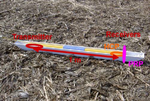
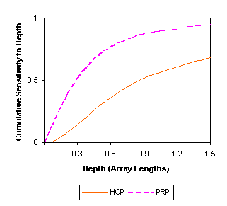
Figure 3 shows an instrument that can practically house a transmitter and several sets of dual HCP and PRP receivers. An instrument with two sets of receivers, e.g. with array lengths of 4- and 1-m or 4- and 2-m, provides four simultaneous measurements of apparent conductivity, each with distinct depth-sensitivity. Such measurements enable the identification of conductive layering in the earth and practical estimation of up to three earth-parameters, e.g. the conductivity of a surficial layer, the thickness of the surficial layer, and the conductivity of the underlying earth.
An instrument with array lengths of 4-, 2- and 1-m provides six simultaneous measurements of apparent conductivity, increasing the robustness of estimates for a 3-parameter earth, or occasionally enabling the analysis of an earth with greater complexity. A shorter instrument, with array lengths of 2- and 1-m, is more convenient for mounting in a sled and yields measurements that are effective for the analysis of a 3-parameter earth within the depths frequently of interest in precision agriculture.
Examples
Three examples show the application of multiple-array measurements to the analysis of layered conductivity. In the first example, the thickness and conductivity of a layer of zero conductivity (air) are estimated, along with the conductivity of the underlying earth, using dual 4- and 1-m arrays.
In the second example, the thickness and conductivity of a loam are estimated, along with the conductivity of underlying bedrock, using dual 4- and 2-m arrays.
In the third example, the thickness and conductivity of freshwater in a lagoon are estimated, along with the conductivity of the sediments at the bottom of the lagoon, using dual 4-, 2- and 1-m arrays.
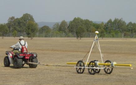
Figure 4 shows the technique of the first example. In the figure, an instrument with dual 1-m arrays is being held at one of a series of heights between on-ground and 2 m.
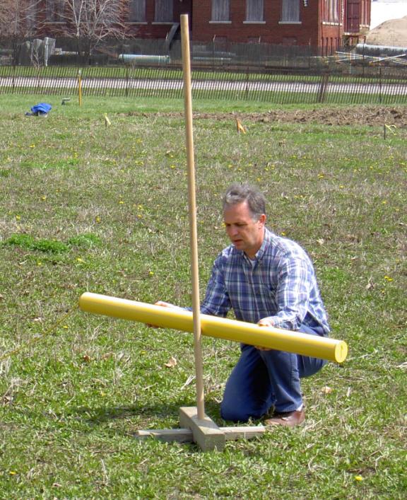
Figure 5 graphs the apparent conductivities measured with the dual 4- and 1-m arrays at a series of heights. All the measurements at the surface are in close agreement at about 25 mS/m, indicating that the earth is highly uniform in conductivity to a depth of several metres.
As the height of measurement increases, the apparent conductivities decrease, as the sensitivities of the arrays lie increasingly in the non-conductive air. Thus, these sets of measurements approximate inverted versions of the cumulative sensitivities shown in Figure 2, with due consideration of the various array-lengths.
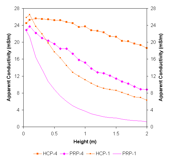
Figure 6 shows the values for layer conductivity, underlying conductivity and layer thickness that, using the sensitivity functions, predicted apparent conductivities that agreed most closely with the measurements plotted in Figure 5. The values were found by a simple Basic-language search routine, and the estimates for layer (i.e. air) conductivity were constrained as non-negative.
The estimated values for underlying conductivity are consistently about 25 mS/m, in close agreement with the at-surface measurements of apparent conductivity. The estimates of layer thickness show excellent agreement with the heights of measurement from surface to 1.3m, and good agreement above that height.
In this example, the underlying earth has moderate conductivity. As suggested by the simulation described later in this paper, the depth range of estimates over more conductive earth might extend beyond 6 m.
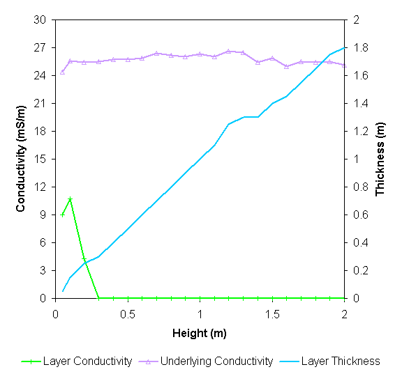
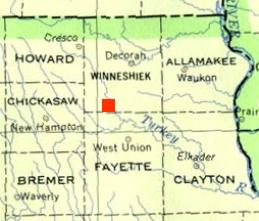
Figure 7 shows the location of the site in north-eastern Iowa of the second example, and figure 8 is a map of the site. The east-west extent of the area is about 250 m. Apparent conductivities were measured at each dot, and the soil was cored at each red dot.
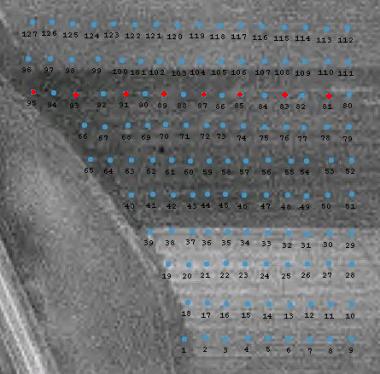
The site is a flat field of well-drained loam overlying carbonate bedrock. The bedrock is exposed in a void near the centre of the western edge of the sampled area.
Figure 9 shows apparent conductivities measured with dual 4- and 2-m arrays on the surface of the loam, along the east-west line with the coring locations. The apparent conductivities are moderate-to-low, yet divergent values for the various arrays suggest the presence of conductive layering. Higher values for the shallower-sensing 2-m PRP array suggest that the conductivity of the soil is higher than that of bedrock.
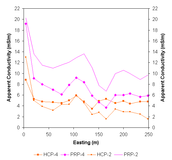
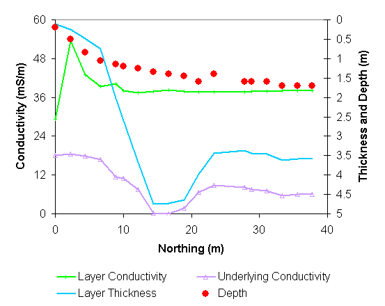
Figure 10 shows the values for a 3-parameter earth that predicted apparent conductivities in best agreement with the measurements plotted in Figure 9. The estimates of layer conductivity range from 12- to 32-mS/m, reasonable for a well-drained loam. The estimates for underlying conductivity are fairly uniform at about 4 mS/m, as might be expected for carbonate bedrock.
The red dots show the soil depth as established by coring. The depths are in good agreement with the estimates of layer thickness, notwithstanding the difference in sampling volume between coring and electromagnetic induction.
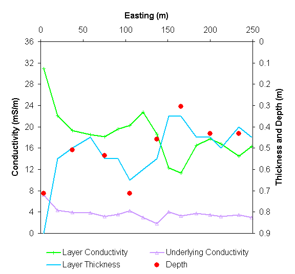
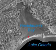
Figure 11 shows the location of the site in Pickering, Ontario, of the third example. Figure 12 shows the survey arrangement on Frenchman’s Bay, a freshwater lagoon.
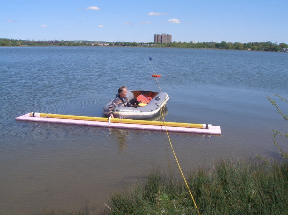
Apparent conductivities from dual 4-, 2- and 1-m arrays were measured on the surface of the freshwater lagoon, and water depths were measured with a sonde. Figure 13 displays the apparent conductivities.
The apparent conductivities are moderate, and decrease as they converge to about 18 mS/m near the shore at 0 N. The convergence probably arises from the increasing proportion of their sampling volumes that is occupied by the saturated sandy material that forms the lagoon barrier.
As water depth increases through first few metres from shore, the apparent conductivities diverge, suggesting the presence of conductive layering.
Further than 10 m from shore the measurements converge, except for those of the 4-m HCP array, which nevertheless rises a few mS/m. Perhaps the water is deep enough in this region to substantially fill the sampling volumes of all but the deepest-sensing 4-m HCP array, which continues to be influenced by less conductive underlying material.
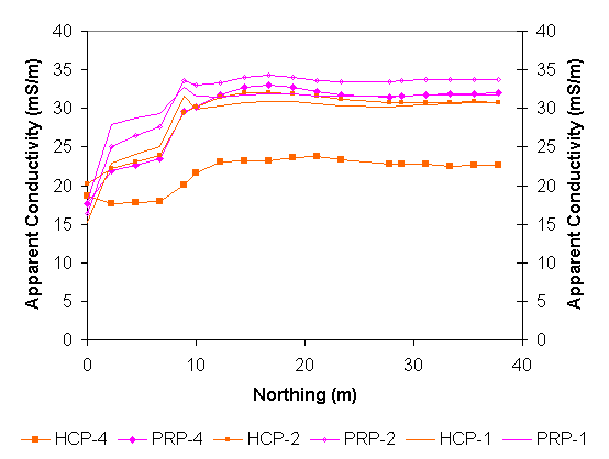
Figure 14 shows the values for a 3-parameter earth that predicted apparent conductivities in best agreement with the measurements plotted in Figure 13. The estimates were found using a “solving” search routine that is an add-in to a popular spreadsheet program. The parameters were constrained as non-negative, and minimum layer-thickness was 0.1 m. Estimates found with the simple Basic-language routine matched the measured depths much better, but the fitting errors were slightly greater.
The estimates of layer conductivity away from shore are about 38 mS/m, somewhat high for fresh water, but reasonable for this lagoon in an urban and industrialized setting. The estimates nearest shore show fluctuation that might arise due to the modest contrast in conductivity between the layer and the underlying earth near the shore. The estimates for underlying conductivity are around 18 mS/m near the shore and decrease to 0- to 7-mS/m under deeper water, values typical of poorly conductive bedrock.
As measured by the depth sonde and indicated by the red dots, water depth ranged from 0.2m nearest shore to a maximum of 1.7 m. Model estimates of layer thickness are in substantial agreement with water depth to about 7 m from shore. Layer-thickness estimates were at a maximum of about 4.7 m 14- to 19-m from shore, beyond which the estimates decreased to about 3.5 m. The thickness estimates might indicate an interface between sediments saturated with lagoon water and resistive underlying material.
Simulation
A widespread application of the EM instruments described herein is the monitoring of soil salinization. This can entail monitoring changes in the depth at which pore-water in a medium-textured soil becomes sufficiently saline to damage vegetation.
To investigate the effectiveness of multi-array instruments for this application, measurements were simulated for an instrument with dual 4-, 2- and 1-m arrays at 0.1-m height over an earth with a layer that ranged in thickness from 0- to 8-m. The layer had a conductivity of 20 mS/m, to represent non-saline medium-textured soil. The underlying earth had a conductivity of 200 mS/m, to represent saline material.
Gaussian error with a standard deviation of ± 1 mS/m was added to the simulated measurements, along with static mS/m offsets of +3 for 1-m HCP, +1 for 1-m PRP, -3 for 2-m HCP, 0 for 2-m PRP, -1 for 4-m HCP and 0 for 4-m PRP. Figure 15 shows the simulated apparent conductivities.
Throughout the range of depths, the apparent conductivities provide at least 5 measurements with reasonable distinctiveness that are at least an order of magnitude above the noise level. This suggests that the measurements from this instrument should be useful for estimating values for a layered earth that has such conductivities and layer thickness.
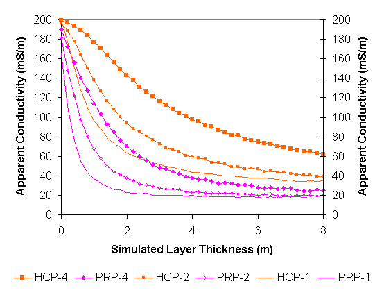
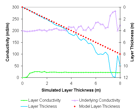
Figure 16 shows the values for a 3-parameter earth that predicted apparent conductivities in best agreement with the simulated measurements. The estimates were found using the “solving” search routine. Local minima in the solution space meant that care was required in the selection of the initial estimates. The parameters were constrained as non-negative.
Where the layer was less than 0.6-m thick, the optimum estimate for layer conductivity was near zero. The estimates for layer thickness, however, and for underlying conductivity were in reasonable agreement with the model. Where the layer was at least 0.6-m thick, the estimates of layer conductivity were reasonable as well.
Estimates of layer thickness and underlying conductivity remained fairly stable until thickness reached around 6 m, beyond which the added noise made these estimates less quantitative.
The static offsets created biases in estimated layer thickness and underlying conductivity that increased with increasing thickness, although the biases did not degrade the estimates as much as the noise did.
Conclusions
Electromagnetic induction with multiple arrays seems capable of producing reliable estimates of layer conductivity, layer thickness and sub-layer conductivity, factors which are important to crop selection and the management of salinity, moisture and nutrients in precision agriculture.
In the examples shown, the data from instruments with multiple array-lengths including 4 m were able to resolve layer thickness to several metres, with an accuracy of a few tenths of a metre where the conductivity contrast was at least moderate.
A simulation where the contrast is an order of magnitude and conductivities are substantially above the noise level suggests that the data were able to resolve thickness to 6 m, and beyond if special care is taken with regard to noise and zero levels. Noise can be reduced by averaging measurements and lengthening the measurement period. Drift in zero levels can be identified through periodic measurements at reference points.
Conductivities estimated for the layer in the simulation show good agreement with the model value where the layer thickness is greater than 0.5 m. The examples suggest similar results were obtained in practice.
Simulated conductivities for the sub-layer appear to be well resolved for layer thickness to 6m, and beyond if special care is take with regard to noise and zero levels. The examples suggest similar results were obtained in practice.
The author acknowledges the assistance of USDA-NRCS staff with the measurements and the provision of coring information for the loam/bedrock example, and the assistance of Geosensors Inc. with the measurements on the freshwater lagoon.
Dualem Products
DUALEM products are used by companies and universities on every continent. Our products fulfill a variety of use-cases in industry and academia.